
机器学习1
定义:
Tom Mitchell : well-posed learning Problem : A computer program is said to learn from experience E whit respect to some task T and some performance measure P, if its performance on T, as measured by P, improves with experience E.
监督学习(supervised learning):
“right answer”given : 给出正确答案, 算法的目的是给出更多的正确答案
回归问题(regression problem)即:设法预测连续值的属性
分类问题(classification problem)即:设法预测一个离散值的输出(如0和1)
无监督学习(unsupervised learning):
“give the algorithm a tons of data and ask it to find structure in the data”给算法海量数据, 找出不同数据的类型结构
聚类算法(clustering algorithms):eg.新闻分类, 找出不同数据之间的联系
鸡尾酒会算法(Cocktail party problem algorithm)eg.音频分离, 找出一个数据中不同的部分
软件:Octave
符号(Notation):
m
Number of training examples(训练样本数量)
“input” variable /features(输入量/特征)
“output” variable /”target” variable(输出量/预测目标变量)
one training example (一个训练样本)
the i ^ th training example(第i个训练样本)
= hypopthesis(假设函数)x,y函数
线性回归(linear regression) / 单变量线性回归 (univariatre linear regression):
θ_i : parameters参数
代价函数(cost function)
代价函数(cost function)是将随机事件或其有关随机变量的取值映射为非负实数以表示该随机事件的“风险”或“损失”的函数。通过最小化代价函数求解最符合的假设函数。
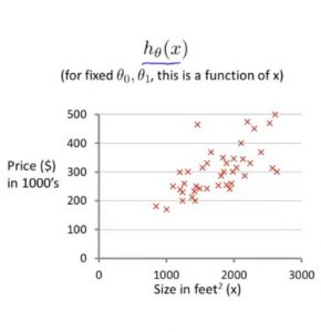
eg.求房子面积(x)和房价(y)之间的假设函数参数
解:
问题变为找到训练集中预测值和真实值的差的平方的和的1/2M倍的最小的θ_0和θ_1的值
定义代价函数:
优化目标:
这个代价函数也叫平方误差函数(squared error function)或者代价平方误差函数(square error cost function)
为什么要求误差的平方和呢?因为误差平方代价函数对于大多数问题, 特别是回归问题, 都是一个合理的选择, 也有其他代价函数也能很好的发挥作用, 但是平方误差代价函数可能是解决回归问题最常用的手段了
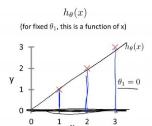
简化假设函数:
得:
代价函数变为:
这里的含义是只选择了经过(0,0)点的函数
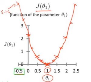
| 假设函数 | 代价函数 |
|---|---|
| 关于参数x的函数 | 关于参数θ_1的函数 |
| x是横坐标 | θ_1是假设函数图像斜率 |
 |
 |
当假设函数变回原来的样子时, 即:
假设函数的图像为:
代价函数的图像变为:
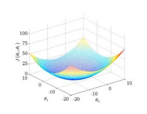
为了方便展示, 常用等高图代替三维表面图
将代价函数J最小化 : 梯度下降算法(gradient descent)
有一个函数:
求:
思路:
给定θ_1,θ_0的初始值, 如都等于0
慢慢接近函数的最小值
重复下面这一步直到收敛:
‘a:=b’表示将b赋值给a
‘a=b’表示断言a和b的值相等
α : 学习率(learing rate),指的是梯度下降时, 每一步的幅度
对于更新方程, 同时更新θ_0和θ_1
何谓同时?
注意: 不能在计算完temp0后马上计算θ_0, 这样算出来的θ_1会被更新后的θ_0所影响.
导数项:
的意义是
函数J()关于 θ_i 的斜率
| 当初始值大于最小值 | 当初始值小于最小值 |
|---|---|
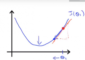 |
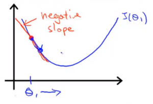 |
| 导数项是正数, θ向最小值移动 | 导数项是负数, θ向最小值移动 |
当θ达到最低点时, 导数项=0, θ不再更新
学习率α的意义是:
θ每次向最小值移动的幅度
| α太大 | α太小 |
|---|---|
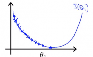 |
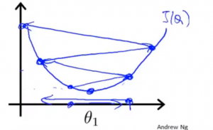 |
| 每次移动的幅度太小, 到达最低点的需要很多步 | 每次移动的幅度太大, 导致无法收敛甚至发散 |
事实上由于斜率在靠近最低点的过程中, 不断地在减少, 所以梯度下降将自动减小每步的幅度
求出偏导项:
\rm{{{\partial \over \partial\theta_j }J(\theta_0,\theta_1)=\frac {\partial}{\partial\theta_j}{1\over 2m}\sum_{i=1}^m(h_\theta(x^i)-y^i)^2}}\\
\rm{={\partial\over\partial\theta_j}{1\over 2m}{\sum_{i=1}^m(\theta_0 + \theta_1x^i-y^i}}\\
\rm{j=0 : {\partial\over\partial\theta_0}J(\theta_0,\theta_1) = \frac{1}{m}\sum_{i=1}^m(h_\theta(x^i)-y^i)}\\
\rm{j=1 : {\partial\over\partial\theta_1}J(\theta_0,\theta_1) = \frac{1}{m}\sum_{i=1}^m(h_\theta(x^i)-y^i)x^i}
\end{aligned}
“Batch”Gradient Desent(Batch下降算法) : each step of gradinet descent uses all the training examples.每一步梯度下降都遍历整个训练集样本
线性代数基础
矩阵(matrix):
\begin{bmatrix}
1 & 2 & 3\\
4 & 5 & 6\\
7 & 8 & 9\\
\end{bmatrix}
(\rm{R^{ 3\times2}})
向量(vector):只有一列的矩阵
\begin{bmatrix}
460\\
232\\
315\\
178\\
\end{bmatrix}
(\rm{R^4})\text{(四维向量集合)}